The Bias-Variance Trade-off
As you get into statistics, you hear people talk about the “bias-variance trade-off” a lot. And when people mention it, they will often start discussing the mean-squared error, which is a function of the bias and variance of an estimator. Then you start looking at formulas. But what does this concept mean intuitively?
To answer this, imagine we have some data \(y_1, y_2, y_3,...,y_n\). The first thing we often want to do is calculate the mean, \(\overline{y} = \frac{1}{n} \sum_{i=1}^n y_i\) and variance \(s^2 = \frac{1}{n-1}\sum_{i=1}^n \left(y_i - \overline{y} \right )^2\). We learn in our first statistics class to get the sample mean we divide by \(n\) but to get the sample variance we divide by \(n-1\); I remember this being terribly confusing. To add to the confusion, if we instead divide by \(latex n\) in our estimate of the sample variance \(\left( \frac{1}{n}\sum_{i=1}^n \left(y_i - \overline{y} \right )^2\right)\), we obtain what is known as the maximum likelihood estimator (MLE) of the variance, which also sounds like a good thing (Maximum! Likelihood!? Sign me up!). We have \(n\) data points, so why don’t we want to divide both the mean and variance by \(n\)?
The reason is that if we divide by \(latex n\) to calculate the variance, our estimate is biased. But will the variance of our estimate also be lower? Yes!
If we repeatedly draw datasets of size 1000 from a Normal(0,1) distribution and calculate the variance for each dataset with both methods, we’ll get a distribution of estimates. With this distribution we’ll get a sense of how much each estimator is biased but also the variance of the estimator. This is what is displayed in figure 1 below. You can see the sampling distribution for both methods with the variance of our estimates given on the figure.
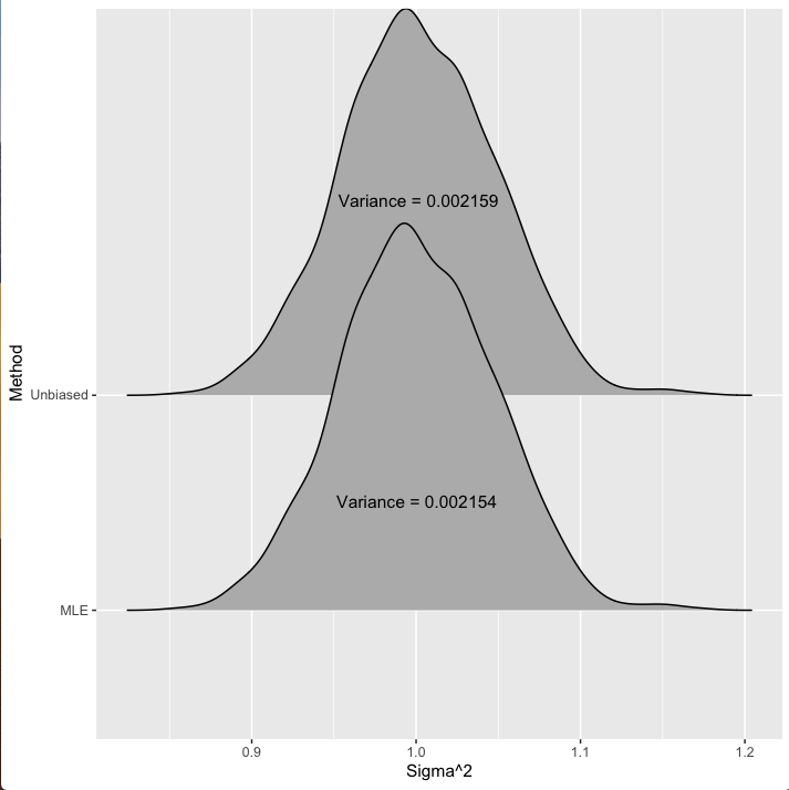 Figure 1: Distribution of the estimates for the variance of 1000 data points drawn from a Normal(0,1) model.
Thus, by introducing some bias we reduce the variance. You can see in figure 1 that this \(n\) vs \(n-1\) doesn’t have much of an effect: the estimate from dividing by \(n-1\) has a variance of about 0.002159, while the estimate of \(\sigma^2\) from dividing by \(n\) has a variance of about 0.002154. Not a huge difference. Similarly, the unbiased estimator (dividing by \(n-1\)) is centered at the correct value of 1 while the MLE estimator (dividing by \(n\)) is centered at 0.999.
A case where the trade-off between bias and variance is easier to see arises in a simple linear regression. The variance around the regression line is usually calculated as \(\hat{\sigma^2}_{\text{unbiased}} = \frac{1}{n-p}\sum_{i=1}^n \left(y_i - \hat{y_i} \right )^2,\) where \(\hat{y_i}\) is the fitted value for observation \(i\) and \(p\) is the number of parameters estimated in the regression. However, the MLE for the same quantity is \(\hat{\sigma^2}_{\text{MLE}} = \frac{1}{n} \sum_{i=1}^n \left(y_i - \hat{y_i} \right )^2\). What effect does using the MLE instead of the unbiased estimator have on our estimates when we have a regression with, say, 500 parameters and 1000 observations?
Let’s assume the variance around the regression line is actually 1. When we repeatedly draw datasets of size 1000 and calculate the variance around the line with both methods, we again get a distribution of estimates and we see the following:
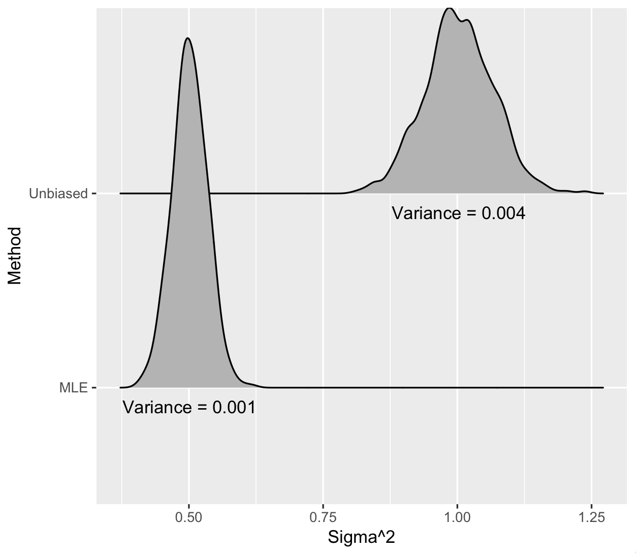 Figure 2: Estimates for the variance around regression line when the true variance is 1. \(n = 1000\) and \(p = 500\).
The MLE does have lower variance—75% smaller—but it is quite biased! The true variance is 1 but the MLE is centered at 0.5. This is an extreme case, since as you get more observations in each dataset relative to the number of parameters, both the MLE and the unbiased estimator look basically the same. But it clearly illustrates the bias-variance trade off.
R Code to replicate this post is below:
#bias variance
rm(list = ls())

require(mvtnorm)
require(doRNG)
require(ggplot2)
require(ggridges)

if (parallel::detectCores() > 1) {
	library(parallel)
	ncores <- detectCores() - 2
	library(doParallel)
	library(foreach)
	library(doRNG)
	registerDoParallel(cores = ncores)
}

nexperiment <- 1000 # number of replications
n <- 1000 # number of observations
p <- 500 # number of parameters
set.seed(11)

#set regression coefficients
beta <- rnorm(p)

output <- foreach(i = 1:nexperiment) %dorng% {
	# data
	X <- rmvnorm(n, sigma = diag(1, p, p))
	Y <- X %*% beta + rnorm(n)

	# model
	fit <- lm(Y ~ X + 0) # add 0 to make sure R does not fit an intercept
	bhat <- fit$$coef

	#variance
	sigma_mle <- sum((Y - X %*% bhat)^2)/n
	sigma_unb <- sum((Y - X %*% bhat)^2)/(n - p)

	Z <- Y/sqrt(sum(beta^2)+1)

	sigma_marg_unb <- sum((Z - mean(Z))^2)/(n-1)
	sigma_marg_mle <- sum((Z - mean(Z))^2)/n

	#output
	return(list(conditional =list(mle = sigma_mle, unbiased = sigma_unb),
	marginal = list(mle = sigma_marg_mle, unbiased = sigma_marg_unb)))
}
# Marginal Variance
sigma_marg_mle <- sapply(output, function(res) res$$marginal$$mle)
sigma_marg_unb <- sapply(output, function(res) res$$marginal$$unbiased)

sigma_df_marg <- data.frame(sigma = c(sigma_marg_mle, sigma_marg_unb), Method = c(rep("MLE", nexperiment),
	rep("Unbiased", nexperiment)))

marg_vars <- paste0("Variance = ",format(c(var(sigma_marg_mle), var(sigma_marg_unb)),digits=4))
E_marg <- c(mean(sigma_marg_mle), mean(sigma_marg_unb))

ggplot(sigma_df_marg, aes(x = sigma, y = Method)) + geom_density_ridges() + xlab("Sigma^2") +
annotate(geom="text", x = E_marg, y=c(1.5,2.9), label = marg_vars)


# Regression Variance
sigma_hat_mle <- sapply(output, function(res) res$$conditional$$mle)
sigma_hat_unb <- sapply(output, function(res) res$$conditional$$unbiased)

vars <- paste0("Variance = ",format(c(var(sigma_hat_mle),var(sigma_hat_unb)),digits=1))
E_sigma <- c(mean(sigma_hat_mle), mean(sigma_hat_unb) )


sigma_df <- data.frame(sigma = c(sigma_hat_mle, sigma_hat_unb), Method = c(rep("MLE", nexperiment),
	rep("Unbiased", nexperiment)))

ggplot(sigma_df, aes(x = sigma, y = Method)) + geom_density_ridges() + xlab("Sigma^2") +
annotate(geom="text", x = E_sigma, y=c(0.9,1.9), label = vars)