WpProj hits CRAN!

This package was quite a mess. It was the first one I’d ever decided to do and filled with na”ivet’e and hubris, I thought it would be a good idea to make a package to load all my functions. It definitely took a long time—especially because a lot of the code was adapting someone else’s C++ code to run for my purpose!—but I think it’s not too bad. There are some places I see that would be obvious places to improve the models but required more work than I currently have time to put in, unfortunately.

What does the package do?

Basically, this package was my round about way of re-inventing \(L_p\) regression. Only slightly kidding. The basic idea is as follows.

Say you have some arbitrarily complex model, \(f\), that takes covariates \(x\), and generates a set of predictions, call them \(\hat{y}\in \mathcal{Y}\), that follow a distribution \(\mu\), with an empirical counterpart \(\hat{\mu}\). Now say this model is really hard to interpret how the \(x\)’s affect the predictions. Let’s say we have another class of models, \(g\), that are easy to interpret. Say these are linear models that typically have the form \(x\beta\). We will denote predictions from this model as \(\hat{\eta}\) and let them have some unspecified distribution \(\nu\) and empirical counterpart \(\hat{\nu}\). (Note that since the \(x\)’s are considered fixed, the distribution is actually coming from the \(\beta\)’s, i.e. \(x\beta \sim \nu\))

It’d be nice if we could use this set of interpretable models from \(g\) to help us understand what’s happening in \(f\). Ideally, these models in \(g\) would be close in some sense to \(f\). We desire

1. Fidelity: predictions from our \(g\) models should be close to \(f\)
2. Interpretability: we should be able to understand what’s happening in \(g\). This also implies our models can’t have too many coefficients.

Let’s address each of these in turn. For 1, we need some way of ensuring predictive distributions are close to one another. One such metric is the \(p\)-Wasserstein distance, defined as

Then we seek to minimize \(\inf_\hat{\nu} W_p(\hat{\mu}, \hat{\nu})^p.\)

Now, for 2. Since the parameter space of \(\hat{\nu}\) could be quite large if the dimensionality of \(x\) is large, then we might not still have an interpretable model—I’d argue that a 1000 covariate regression model is not, in fact, interpretable!

Going back to our minimization problem, we want to add some kind of penalty for large parameter distributions

We should note that \(\hat{\nu} = x \hat{\beta}\). So, we need someway of reducing the dimensionality of the \(x\)’s. But fortunately, for linear models there’s a decades old method of doing just that!

Rather than focusing on the \(x\)’s, we focus on reducing the dimensions of \(\beta\) using a penalty like the group Lasso:

Finally, if we let the number of atoms in empricical distributions be equal, then the problem will reduce to

Cool!

Let’s see an example

Ok, say we have some covariate data, \(X\), and an outcome, \(Y\). In many cases, the size of \(X\) can be quite large—in the 100s or 1000s. The question of then how to interpret this model can be tough: what covariates do we focus on? Moreover, the model itself may not be interpretable to begin with, such as from a Gaussian Process, a neural network, etc.

Estimating a data model

For exposition, we will generate our data from a hard to interpret, non-linear model and then fit a Bayesian Gaussian Process regression to estimate the response surface. The set-up will be somewhat complicated but it’s basically to generate complicated data and fit a complicated model.

First, let’s assume our data is drawn from the following distributions. Let \(K = 10\) and \(N = 1000\). Take

and

where \(\epsilon_{1:N} \sim \mathcal{N}(0,1)\). The function $f$ is defined as

We can generate the parameters of this generating function by taking \(\alpha_0, \alpha, \delta \sim \mathcal{N}(0,1)\) and \(\epsilon_{1:N} \sim \mathcal{N}(0,1)\)

Then, assume for some reason we know the true model (this is so we can run all of the methods for our package). And we will fit a Bayesian regression model directly on this model.

We can assume normal priors on the coefficients (which will be the same as the data generating process above), and a half-normal prior on the standard deviation: \(\sigma \sim \mathcal{N}^{+}(0,1)\)

We can then fit this model with the following R code:

library(rstan)

# Simulated Data
set.seed(42)
N <- 2^10
K <- 10

# parameters
alpha_delta <- rnorm(K + choose(K,2))
alpha_0 <- rnorm(1)

# data
x <- matrix(rnorm(N * K), N, K)
mm<- model.matrix(~ 0 + .*., data = data.frame(x))
y <- c(mm %*% alpha_delta + alpha_0 + rnorm(N))

code <- '
data {
  int N;
  int K;
  vector[N] Y;
  matrix[N,K] X;
}
parameters {
  vector[K] alpha;
  real<lower=0> sigma;
  real alpha_0;
}
model {
  vector[N] mu_raw = X * beta + beta_0;
  
  alpha0 ~ normal(0,1);
  alpha ~ normal(0,1);
  sigma ~ normal(0,1);
  Y ~ normal(mu_raw, sigma);
}
generated quantities {
  vector[N] mu = X * beta + beta_0;
}
'

fit <- stan(model_code = code, 
            data = list(N = N, K = ncol(mm), Y = y, X = mm),
            iter = 500, chains = 4, cores = 4)

Interpretable model

We can estimate an interpretable model, which essentially ammounts to fitting regression to the samples. How we do this can vary for our methods. Since we know the true model, we may simply seek to turn the covariates on our off and get our set of interpretable coefficients. Alternatively, we may want to find an approximate model with new coefficients. We can do both in the framework briefly described above. The basic idea is to find coefficients such that \(\hat{\nu} = f_\beta(X)\) is as close as possible to \(\hat{\mu}\). However, it is important to consider what we want to interpret.

We could want to know how the model roughly functions globally, or which covariates could be the most important, but we may also want to know which covariates are driving the prediction for a single individual and consider the most important ones.

Let’s say we’re interested in the 5th individual in our data. We can pul their data

X_mm  <- cbind(1,mm)
X_test <- X_mm[5,]

And then we can run our interpretable models. We first run our set that can get interpretable models for a single data point–i.e., by simply turning coefficients on or off that best predict the data. The details are explained more fully in the paper, but basically for \(W_2\) distances, we can represent the problem as a binary program:

library(WpProj)

# get parameters
mu <- extract(fit, pars = "mu")$mu
beta <- do.call("cbind", extract(fit, pars = c("beta_0","beta")))

# get prediction
mu_test <- mu[,5]
  
# get interpretable models            
bp <- WpProj(X = X_test, eta = mu_test, theta = beta,
             power = 2, method = "binary program",
             solver = "ecos",
             options = list(display.progress = TRUE))

approx <- WpProj(X = X_test, eta = mu_test, theta = beta,
                 power = 2, method = "binary program",
                 solver = "lasso",
             options = list(display.progress = TRUE))

We can also fit a model that simply finds a lasso regression closest to \(\hat{\mu}\). To do so, we need to create a pseudo neighborhood round our point of interest

library(mvtnorm)

pp <- ncol(mm) 

# generate the neighborhood arround the point
X_neigh <- mvtnorm::rmvnorm(100, mean = X_test[-1], sigma = cov(X_mm[,-1])/N)

# get predictions for the neighborhood
mu_neigh <- cbind(1,X_neigh) %*% t(beta)

# get projection
proj <- WpProj(X = cbind(1,X_neigh), eta = mu_neigh, 
               theta = beta,
               power = 2, method = "L1",
               solver = "lasso")

Performance Evaluation

For our individual, they have an average predicted value of -6.7314591.

# Check WpR2
rp <- WpProj::ridgePlot(fit = list("BP" = bp,
                                    "approxBP" = approx,
                                    "projection" = proj),
                          full = mu_test
                          )

print(rp)

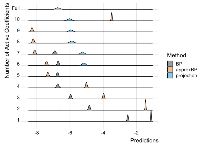
We can see that the interpretable models do a better job of predicting as covariates are added but we might need more than just 10 covariates to really do a good job here.

# Check WpR2
wpr2 <- WpProj::WPR2(predictions = mu_test,
             projected_model = list("BP" = bp,
                                    "approxBP" = approx,
                                    "projection" = proj),
             base = rep(0, 1000))

plot(wpr2)

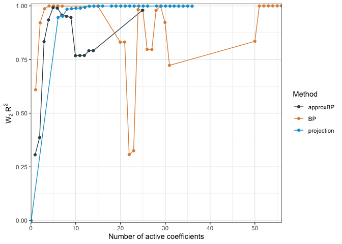
This last statistic functions kinda like \(R^2\) values in regression except it is measuring how close an interpretable model is to the full model as compared to a null model, such as one with just the intercept:

If the null model is appropriately chosen, this quantity \(W_p R^2\) will be in \([0,1]\), but can be negative if not.

Extensions

One obvious extension is to have arbitrary transformations of the preditive function \(x\beta\). This would be useful in the case where we have something like predictions on a probability space and we want our coefficients to be selected such that they do the best job of predicting on that space rather than the linear predictor space:

This may also allow the models to have uses in other applications, which hopefully I will be working on soon!

Where can I find the latest version of the package?

As always, on my Github. For more links, check out the repositories page on this site.